
APVT-590 Air PVT Panels: From Rated Power to Useful Heat for Workshop Ventilation
Connect APVT-590 ratings to the ventilation airflow, useful temperature rise, operating schedule and fan energy that determine the heat a workshop can actually use.
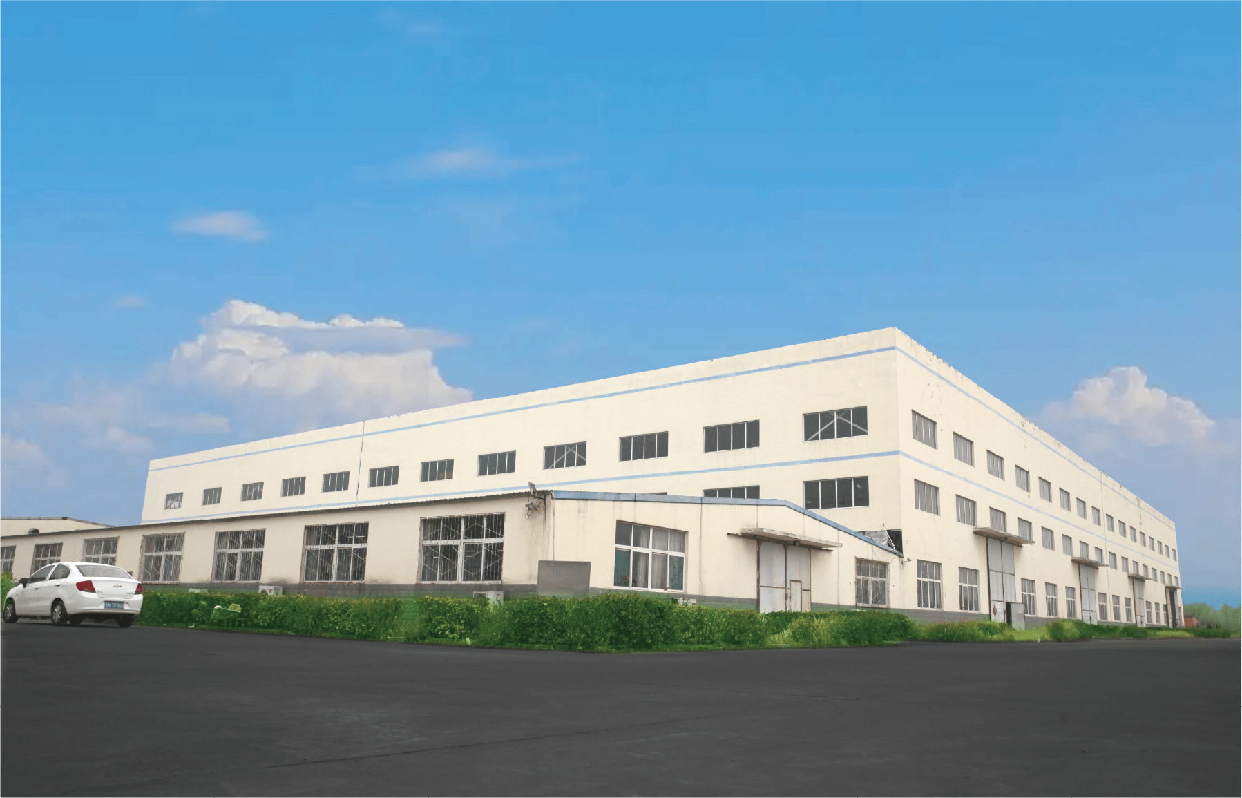
A workshop can have a sunny roof, a substantial ventilation heating bill and very little use for hot water. An air PVT panel is worth evaluating in that situation because its thermal output arrives as warm air, while its photovoltaic section supplies electricity. The important question is how much of that warm air the building can use during its operating hours.
The answer cannot come from multiplying the panel’s peak thermal power by the length of the working day. A useful proposal must connect five quantities: actual airflow, temperature rise, distribution losses, the heating demand at that moment and the electricity needed to move the air.
This guide applies that approach to the SOLETKS APVT-590. It is intended for ventilation contractors, workshop owners and project buyers comparing an air PVT installation with their existing fresh-air heating arrangement.
What the APVT-590 ratings tell a buyer
The SOLETKS Air PVT product page identifies APVT-590 as a hybrid panel for electricity and warm-air applications. Its public data provides a starting point, but several entries need a common measurement basis before they can become a system forecast:
| Published item | Listed value | Interpretation for a proposal |
|---|---|---|
| Electrical maximum power | 590 W under STC | A PV test rating, not continuous site output |
| Listed module efficiency | 23.3% | Requires confirmation of the reference area and product revision |
| Outline dimensions and area | 1,148 × 2,293 × 80 mm; 2.63 m² | Physical space information; the efficiency reference area still needs checking |
| Peak thermal power | 1,551 W | A thermal rating requiring its test conditions |
| Peak thermal efficiency | 0.59 | Cannot automatically be combined with the electrical peak |
| Airflow | 70–90 m³/h | A starting range to confirm for the selected module arrangement |
| Static pressure | 120 Pa | An entry whose measurement boundary must be clarified |
| Power temperature coefficient | −0.28% per °C | Relates PV power to cell temperature under the stated rating convention |
These entries should not automatically be treated as one simultaneous operating point. The public table does not establish that the peak heat rating occurs at every airflow in the stated range. Nor does the pressure entry establish the fan pressure available for the complete building duct network.
Ask for the thermal performance curve and the pressure-loss curve, including their airflow, temperature and test conditions. The distinction between collector testing and complete-system performance is also reflected in IEA SHC Task 60’s PVT performance and modelling work.

Three arithmetic checks before accepting a yield estimate
Electrical area check. At the STC irradiance of 1,000 W/m², 590 W divided by the listed 2.63 m² outline area gives 22.4%, rather than 23.3%. Conversely, 590 W at 23.3% implies a reference area of approximately 2.532 m². A different area definition or product revision could explain the difference, but the public page does not resolve it. The quotation should identify the matched power, area and efficiency; it should not silently combine them.
Thermal area check. The ratio 1,551 ÷ (1,000 × 2.63) is approximately 59.0%. Those values are arithmetically consistent if the thermal test uses that irradiance and area. This calculation does not establish that those were the actual test conditions, or that electrical and thermal peaks occurred simultaneously.
Air-temperature check. Using the air properties defined below, transferring 1.551 kW into 80 m³/h would require approximately 57.9 K of temperature rise. That is a consistency calculation, not a promised outlet temperature. It shows why the listed airflow and peak heat cannot be treated as a complete operating point without the test inlet temperature, irradiance and measurement boundary.
These checks do not establish that the product cannot perform as listed. They identify the missing information needed to turn a catalogue into an engineering selection.
What the rest of the product sheet adds
The remaining electrical and construction data supports several further checks:
| Published entry | ค่า | Consequence for the design |
|---|---|---|
| Cell construction | 144 N-type TOPCon monocrystalline cells | Identifies the listed PV construction; does not establish an annual yield |
| Vmp / Imp | 44.45 V / 13.27 A | Their product is 589.9 W, consistent with the 590 W rating |
| Voc / Isc | 51.1 V / 14.31 A | Gives a fill factor of about 0.81 when compared with 590 W |
| Maximum system voltage | 1,500 V | String design also needs cold-corrected Voc and inverter limits |
| Operating temperature | −40 to 70°C | The supplier must identify whether this means ambient, module or another component temperature |
| Air connections | Two Ø100 mm interfaces | Local velocity and fitting losses matter at each module |
| Weight / cover | 37 kg; 3.2 mm glass | About 14.1 kg/m² of outline area before frames and ductwork |
| Connector / fire entry | MC4; IEC fire class C | Confirm the actual connector pairing and the applicable fire-test standard and assembly scope |
| Packing | 12 units per pallet; 240 per 40 ft container | Relevant to logistics, separate from operating performance |
Fill factor here means Pmax/(Voc × Isc). It is an electrical consistency check, not an efficiency measurement. The published power temperature coefficient is also insufficient for cold-voltage string sizing: that task requires the voltage coefficient and the electrical manufacturer’s design instructions. Likewise, the fire-class entry by itself is not approval of a roof-and-duct assembly.
The air connection creates a local velocity. If one Ø100 mm opening carries the full 80 m³/h module flow, its area is 0.00785 m² and velocity is 2.83 m/s, increasing to 3.18 m/s at 90 m³/h. At the assumed density of 1.20 kg/m³, the velocity pressure at 80 m³/h is ρv²/2 ≈ 4.8 Pa. A fitting with local loss coefficient ζ adds approximately ζ × 4.8 Pa at that velocity. This is not the total panel pressure drop. If the two ports are the inlet and outlet, their areas must not be added as though they were parallel inlets.
At 800 m³/h total, an assumed clear-bore Ø250 mm header carries air at about 4.53 m/s; Ø315 mm gives 2.85 m/s. These velocities are comparisons, not selected duct sizes. Header resistance and its distribution along the array affect branch balance as well as fan energy.
The thermal peak and temperature range need a common definition. Combining 1,551 W, 80 m³/h and a 20°C inlet using the constant-density approximation gives an outlet near 78°C. That exceeds the number 70°C in the table, but outlet air temperature is not necessarily the temperature to which the listed limit applies. The calculation therefore raises a question rather than proving a contradiction. A zero-temperature-difference efficiency intercept or a different test flow could explain the peak figure; neither explanation is confirmed by the page. Obtain the test point and the temperature-limit definition together.
The claimed lifetime PV improvement needs a comparison baseline. The product page mentions a possible 10–15% improvement in photoelectric performance over the life cycle under suitable conditions. If 10–15% were interpreted as a gain normalized to the same reference power and irradiance, the linear −0.28%/K coefficient would imply approximately 36–54 K of cell cooling. An annual relative gain against a hotter reference module is not calculated in exactly that way: its denominator and irradiance-weighted temperature history matter. The claim needs the reference module, climate, operating airflow and definition of “performance”; it should not be inserted into a financial model as a guaranteed annual uplift.
Start with the ventilation duty the workshop already needs
- Outdoor intake
- Filtration
- Solar air path or bypass
- Backup heating
- Occupied space
Ventilation must remain available during cloud, excess solar heat and a solar-system fault. Fan location and protection require a project-specific design.
Consider the heating required to bring outdoor replacement air to an acceptable supply condition. Identify the existing air path before selecting a panel quantity:
Outdoor intake → filtration → solar air path or bypass → backup heating → occupied space.
This is a functional sequence, not an installation drawing. The designer must decide the fan location, permitted air paths, fire provisions and the relationship to any existing heat-recovery equipment.
Three questions make the product assessment much more specific:
- Is ventilation operating when sunlight is available? A daytime workshop has a different opportunity from a facility whose largest heating requirement occurs before sunrise.
- Is this genuinely additional heat? If an existing heat-recovery unit already warms the incoming air, evaluate the solar contribution against that actual baseline. Counting both systems as heating air independently from outdoor temperature overstates the benefit.
- Can the building accept the air? Required outdoor-air delivery must continue during cloudy weather, excess solar heat and a solar-system fault. A bypass and backup arrangement should preserve that function.
Solar ventilation preheating reduces the heating required after outdoor air enters a building. The WBDG Solar Ventilation Air Preheating reference addresses this application. APVT adds photovoltaic generation to the thermal task, while the ventilation designer still has to establish the complete air path and operating baseline.
For a workshop with process exhaust, establish the replacement-air requirement with the ventilation designer. Contaminated exhaust air is not interchangeable with a clean solar intake or an unrestricted recirculation stream.

Calculate heat from airflow and temperature rise
For a sensible-heating estimate:
Heat rate = air mass flow × air specific heat × temperature rise.
Using airflow in m³/h, an assumed air density of 1.20 kg/m³ and specific heat of 1,005 J/(kg·K):
Q = 0.000335 × V × ΔT
where:
- Q is heat rate in kW;
- V is volumetric airflow in m³/h at the condition used for the density assumption;
- ΔT is outlet minus inlet air temperature in °C or K.
For example, an assumed 80 m³/h passing through a panel and gaining 20 K carries:
Q = 0.000335 × 80 × 20 = 0.536 kW.
This is a calculation for an assumed operating condition, not a measured APVT-590 result or a prediction derived from its peak rating. Actual density changes with altitude and temperature. Where humidity changes, condensation or another latent process matters, the engineer should use a moist-air enthalpy balance instead of this sensible-only approximation.
A hot outlet is not sufficient evidence of high useful output. A restricted air path can produce a noticeable temperature rise while moving too little air to carry much heat. Measure or calculate airflow and temperature together.
Why flow changes both temperature and collection efficiency
As a first arithmetic comparison, suppose the same 0.536 kW enters the air at three different flows:
| Assumed flow per panel | Temperature rise carrying the same 0.536 kW |
|---|---|
| 70 m³/h | 22.9 K |
| 80 m³/h | 20.0 K |
| 90 m³/h | 17.8 K |
The highest outlet temperature in this table carries no more heat than the lowest. The heat rate was deliberately held constant to isolate the effect of airflow.
A real collector does not necessarily hold that heat rate constant. Airflow changes convection inside the passage, absorber and cell temperatures, and heat loss to the surroundings. At approximate steady state, absorbed solar energy divides among electricity, useful air heating and external heat loss; during warm-up, some also increases the panel’s stored thermal energy. A low-flow, high-temperature operating point may therefore collect less heat while demanding less fan power. A higher-flow point may collect more heat but incur a larger electrical penalty. The measured thermal and resistance curves are needed to locate the useful operating range.
Air density is another source of error. If actual density is 1.00 rather than 1.20 kg/m³, the calculated heat at the same actual volumetric flow and temperature rise is 16.7% lower. Standardized airflow and actual airflow must not be inserted into the same equation without reconciling their density basis.
A simple loss model explains the difference between a peak and a working point
For an illustrative steady-state collector with inlet air at ambient temperature, assume:
Q = A × G × η₀ − A × a₁ × (Tm − Ta),
Tm − Ta ≈ ΔT/2, และ Q = C × ΔT.
Q is in watts; C = 0.335 × V is the air heat-capacity rate in W/K for V in m³/h under the earlier property assumptions. Solving gives:
ΔT = A × G × η₀ ÷ (C + A × a₁/2).
Take A = 2.63 m², an assumed η₀ of 0.59, and an assumed a₁ of 8 W/(m²·K). The first number is chosen to illustrate a possible interpretation of the published peak efficiency; it has not been verified as the APVT curve intercept. The second is a sensitivity input, not a published APVT loss coefficient.
| Flow per module | Rise at 1,000 W/m² | Heat at 1,000 W/m² | Rise at 700 W/m² | Heat at 700 W/m² | Model efficiency at either irradiance |
|---|---|---|---|---|---|
| 70 m³/h | 45.7 K | 1,071 W | 32.0 K | 750 W | 40.7% |
| 80 m³/h | 41.6 K | 1,114 W | 29.1 K | 780 W | 42.4% |
| 90 m³/h | 38.2 K | 1,150 W | 26.7 K | 805 W | 43.7% |
Within these assumptions, useful heat at 1,000 W/m² remains below the approximately 1,552 W zero-loss term A × G × η₀ because warming the air creates a loss term. Higher flow increases collected heat while reducing outlet temperature. This demonstrates a mechanism; it does not establish an APVT performance curve or a temperature-safe operating point. Real heat removal, coefficients and air properties can change with flow and temperature.
For a PVT test, the electrical state also belongs in the report. Operation at maximum power point exports electrical energy, while an open-circuit test has a different energy balance and module temperature. Thermal results should identify that state before being combined with an electrical forecast.
A worked example: ten panels serving a daytime ventilation branch
The following example is deliberately hypothetical. It demonstrates the calculation method; none of the assumed temperature rises or losses is an APVT-590 performance guarantee.
สมมติ:
- Ten modules in a manufacturer-approved parallel air arrangement.
- Balanced flow of 80 m³/h per module, giving 800 m³/h total.
- Outdoor inlet air at 5°C during the illustrated periods.
- A ventilation supply target of 20°C, requiring a maximum useful solar rise of 15 K.
- Ninety percent of the collected sensible heat reaches the backup-heater inlet.
- The workshop uses this ventilation branch throughout the seven illustrated hours.
At 800 m³/h, the air stream carries 0.268 kW per kelvin of temperature rise. Its heating requirement from 5°C to 20°C is therefore:
0.268 × 15 = 4.02 kW.
That requirement places a ceiling on the solar heat this branch can use at that moment.
| Illustrative period | Duration | Assumed collector air-temperature rise | Heat reaching the backup-heater inlet after the assumed loss | Useful solar energy accepted by the load |
|---|---|---|---|---|
| Morning | 2 h | 8 K | 1.930 kW | 3.86 kWh |
| Midday | 3 h | 20 K | 4.824 kW, capped by the 4.02 kW load | 12.06 kWh |
| Afternoon | 2 h | 12 K | 2.894 kW | 5.79 kWh |
| Total | 7 h | — | — | 21.71 kWh |
Before distribution losses and the load ceiling, the collector-side calculation produces 26.80 kWh. After the assumed distribution loss, 24.12 kWh reaches the ventilation equipment. Only 21.71 kWh replaces useful heating in this example because the midday solar contribution exceeds the specified ventilation heating requirement.
This difference matters when comparing proposals. A quotation based on collector output alone would count heat the load cannot accept. A control strategy might redirect some excess heat to another real load, but that load and its ductwork must exist before the energy can be credited.
At midday, the ventilation arrangement must regulate supply temperature while maintaining required airflow. Simply reducing the workshop’s fresh-air supply until the outlet temperature looks attractive is not an acceptable performance improvement.
When the workshop needs more air than the solar branch supplies
The entire ventilation flow does not necessarily have to pass through collectors. A solar branch can preheat part of the outdoor air and mix with a bypass stream, provided the air-handling design permits that arrangement.
Consider a separate hypothetical operating point: the workshop needs 2,400 m³/h, but the ten-panel branch handles 800 m³/h. Outdoor air is 5°C and solar-branch air leaves the collectors at an assumed 35°C. If 90% of the collected temperature rise survives distribution, solar air reaches the mixing point at:
5 + 0.90 × (35 − 5) = 32°C.
With the other 1,600 m³/h bypassing at 5°C, and using a common air-density approximation, the mixed temperature is:
Tmix = (800 × 32 + 1,600 × 5) ÷ 2,400 = 14°C.
The load and contribution then become:
| Quantity | การคำนวณ | Result |
|---|---|---|
| Heating all outdoor air from 5°C to 20°C | 0.000335 × 2,400 × 15 | 12.06 kW |
| Solar heat delivered through the smaller branch | 0.000335 × 800 × 27 | 7.236 kW |
| Backup duty after mixing | 0.000335 × 2,400 × (20 − 14) | 4.824 kW |
This explains why a 35°C collector outlet does not mean the workshop receives 35°C supply air. It also shows how a relatively small solar branch can make a measurable contribution without reducing required ventilation. For an exact balance, use mass flows and moist-air properties for the two streams.
The mixing point matters if heat recovery already exists. Solar air entering upstream of a recovery exchanger changes its temperature difference and may displace some recovered heat; solar downstream of it faces a warmer inlet condition. Compare the proposed sequence against the same building, airflow and heat-recovery controls with solar bypassed. Crediting the full solar rise from outdoor temperature on top of unchanged recovery can double-count heat.
Match panel arrangement to airflow, not only roof area
Ten air collectors do not behave like ten electrical modules in a string. The electrical and air-side arrangements must each be designed.
With parallel air branches, their flows add at the common duct, but branch resistance and balancing determine whether every collector receives the intended flow. The fan pressure is based on the controlling flow path and shared duct sections; it is not ten times the pressure drop of one identical parallel branch.
With collectors in series, the same air passes through successive modules. Inlet temperature rises along the path, pressure losses accumulate and downstream collectors operate under different thermal conditions. A series arrangement therefore cannot be evaluated by simply adding independent peak ratings.
Request the approved number of modules per branch, connection arrangement and balancing method. A drawing should identify the longest or most restrictive air path, the clean-filter condition and the expected filter-loading condition.
For the broader choice between direct-air equipment and a liquid loop feeding an air coil, use the separate solar air heating architecture guide.
Account for fan electricity separately
The air has to overcome resistance from the collector, ducts, bends, filters, dampers and other components. Fan selection should use a complete duty point and a consistent pressure definition. The DOE fan-system sourcebook explains the relationship between airflow, pressure and fan power, and why the installed duct arrangement affects performance.
An approximate electrical-input calculation is:
Fan input = volume flow in m³/s × fan total-pressure rise in Pa ÷ overall efficiency.
For illustration, assume a complete duty of 800 m³/h at 250 Pa, with combined fan, motor and drive efficiency of 0.50:
P = (800 ÷ 3,600) × 250 ÷ 0.50 = 111 W.
Seven hours at that input would consume approximately 0.78 kWh. These are assumed fan-system values; the 250 Pa is not inferred from the APVT product-page pressure entry.
The resistance penalty grows faster than airflow
For an unchanged duct network dominated by turbulent friction, pressure drop is approximately proportional to flow squared. If overall fan efficiency stays similar, electrical input consequently scales approximately with flow cubed. Dampers, filter loading and changes in efficiency can alter that relationship.
For a separate assumed network requiring 300 Pa at 800 m³/h and an overall efficiency of 0.45:
| Total flow | Approximate network pressure drop | Calculated fan input |
|---|---|---|
| 700 m³/h | 230 Pa | 99 W |
| 800 m³/h | 300 Pa | 148 W |
| 900 m³/h | 380 Pa | 211 W |
A 12.5% flow increase from 800 to 900 m³/h therefore increases fan input by about 42% in this example. It would need a useful thermal or ventilation benefit to justify it. These are network calculations, not an APVT pressure-loss curve. The actual operating point is where the selected fan characteristic meets the installed system resistance.
For the energy comparison, distinguish the total fan input from the increase caused by adding the solar path. A workshop that already needs a ventilation fan should normally compare the modified installation with its existing airflow and fan consumption. Charging all fan electricity to solar may overstate the added consumption; ignoring the new resistance understates it.
Also distinguish heat from electricity. If the 21.71 kWh of useful heat in the example displaced a heater operating at an assumed COP of 3, it would avoid approximately 7.24 kWh of heater electricity. Allocating the full illustrative 0.78 kWh fan consumption to solar leaves approximately 6.46 kWh of net heating-electricity reduction, before other controls or losses. A different backup system requires a different conversion.
PV generation remains a separate electrical contribution. Do not treat nominal PV watts as measured daily energy, and do not credit the same PV electricity once as exported generation and again as electricity consumed by the fan. If downstream air-temperature measurements include fan heat, separate that contribution when reporting solar thermal performance.
The published temperature coefficient also needs the right temperature. At the same irradiance, a simple correction from 25°C to an assumed 55°C cell temperature gives 590 × [1 − 0.0028 × (55 − 25)] ≈ 540 W before other electrical losses. Air outlet temperature is not cell temperature, so it cannot be substituted into that calculation. Assess annual PV yield with cell-temperature behaviour, shading, wiring and inverter losses as well as irradiance.
Does fan operation for PV cooling alone save electricity?
If the approved system can exhaust warm air outdoors when there is no heating demand, compare the extra PV electricity with the extra fan electricity. Using the published coefficient, the simplified electrical gain per kelvin of cooling is:
590 × 0.0028 × (G/1,000) W per module.
At G = 800 W/m², this is about 1.32 W/K. An assumed 10 K cell-temperature reduction across ten modules would produce approximately 132 W of extra DC power. If solar cooling adds the full 111 W fan input from the earlier example, the difference is only about 21 W, even before conversion and control losses. If part of that fan consumption was already required for ventilation, compare only the increment.
The example explains why a thermal benefit and a PV-cooling benefit must be evaluated separately. Neither the 10 K cooling effect nor a positive summer balance is demonstrated by the product table. Any cooling mode also needs an approved exhaust or bypass path and a credible comparison with the uncooled electrical baseline.
Heat recovery, operating days and air quality set the usable opportunity
Stable daytime outdoor-air demand gives solar heat an immediate load. Existing heat recovery and high internal heat gains can reduce the remaining heating requirement. A controlled bypass should preserve ventilation when the solar path is unhelpful; it should not force unwanted heat into the workshop.
The work calendar can be as important as collector area. In an intentionally uniform seven-day example, removing two otherwise identical operating days removes 2/7, or 28.6%, of the potential operating opportunity. This is calendar arithmetic, not an annual savings factor: real weather, holidays, start times and demand vary. Model those periods rather than applying a universal weekend discount.
Specific airflow also prevents misleading comparisons. A reference design at 4 cfm/ft² corresponds to 73.15 m³/h per m². APVT at 80 m³/h over its 2.63 m² outline operates at approximately 30.42 m³/h per m², about 42% of that reference flow. A rule intended for an unglazed transpired collector should therefore not be transferred to this panel. At equal useful heat per area, lower specific airflow would give a larger temperature rise; different collector efficiencies mean equal heat per area cannot simply be assumed.
At night, a collector channel can cool below outdoor-air temperature. The designed bypass should then maintain the required ventilation while avoiding an unwanted cooling path, subject to the product’s operating requirements. Include filter loading in the resistance calculation. For drying or recirculation, assess the actual humidity and air cleanliness: humid return air can introduce condensation, while dust can affect pressure loss and hygiene. Those are different duties from heating clean outdoor air.
Controls determine whether the warm air has value
A practical operating description should cover the following states:
| Operating condition | Required outcome |
|---|---|
| Sun available and the workshop needs heat | Admit useful solar air while maintaining ventilation duty |
| Solar air warmer than the permitted supply condition | Mix, bypass or modulate through an approved arrangement |
| Cloud or low collector temperature | Maintain ventilation and let backup heating complete the duty |
| No heating demand | Preserve ventilation without forcing unwanted solar heat indoors |
| Fan, sensor or damper fault | Follow the designed fault mode and maintain the required building function |
| Electrical generation available without thermal demand | Operate only within the panel’s approved airflow and temperature conditions |
Do not assume that the last state is automatically harmless. Obtain the manufacturer’s requirements for no-flow operation and high-temperature protection, and coordinate them with the electrical design.
For a heat-pump backup, a useful additional control check is whether Quseful ÷ COP exceeds the incremental fan input. At an assumed COP of 3, an extra 60 W of fan electricity requires more than 180 W of useful thermal displacement to reduce total heating electricity. Use consistent units and the actual backup operating condition. Required ventilation and any manufacturer-required panel cooling still take priority over this energy-saving test. Start/stop delays and suitable hysteresis also matter under passing clouds; a momentary positive temperature difference is not sufficient reason to cycle dampers and fans continuously.
Measure a heat balance, including its uncertainty
A commissioning record should establish inlet and outlet temperatures, actual airflow, irradiance in the panel plane, fan electricity, outdoor conditions and damper state on the same time basis. Put the thermal measurement boundary where its meaning is clear: across the collector for collector heat, or at the building connection for delivered heat. Mixing, air leakage, duct losses and fan heat between those boundaries explain why the two results differ.
Measure representative bulk air temperatures. A sensor touching warm ductwork, sitting in direct radiation or sampling an unmixed hot streak can exaggerate the rise. Likewise, a single velocity reading at the centre of a duct is not necessarily its average flow. Measurements during thermal warm-up should not be presented as steady performance.
The effect of a small temperature difference can be quantified. Suppose an illustrative measurement system has independent standard uncertainties of 5% in airflow, 2% in density and 0.3 K in each temperature measurement. Neglecting specific-heat uncertainty, root-sum-square propagation gives:
uQ/Q ≈ √[(0.05)² + (0.02)² + (√2 × 0.3 ÷ ΔT)²].
| Measured temperature rise | Approximate relative standard uncertainty in heat rate |
|---|---|
| 4 K | 11.9% |
| 20 K | 5.8% |
These are illustrative uncertainty assumptions, not the accuracy of a named instrument. A manufacturer’s “±” specification cannot automatically be treated as a standard uncertainty. Correlated sensor errors, leakage and unrepresentative sampling need separate treatment. The practical implication is that a small claimed gain at low temperature rise can be indistinguishable from measurement error unless the measurement arrangement is adequate.
For seasonal energy, perform the load-capped calculation at each time step:
Euseful = Σ max[0, min(Qdelivered, Qheating demand)] × Δt.
Use operating hours, local weather, the actual heating baseline and the collector performance map at the relevant inlet temperature and flow. If the workshop is closed, the heating demand may be zero even on a sunny day. If another load accepts surplus heat, model its temperature requirement and availability explicitly. This turns a peak rating into a defensible estimate of heat the business can use.
What a useful APVT proposal should contain
Send SOLETKS the project location, required outdoor airflow, working hours, desired supply condition, current heating arrangement, available installation area and a sketch of the duct route. Include existing heat recovery, filtration and process-exhaust requirements where relevant.
Ask the proposed system to return four connected results:
- Air duty: module arrangement, flow per branch and complete fan duty.
- Thermal contribution: useful heat at the building connection over the operating schedule, with assumptions and losses stated.
- Electrical contribution: PV forecast and auxiliary electricity reported separately.
- Operating method: bypass, backup, overtemperature and fault responses.
At commissioning, compare those calculations with airflow, temperatures, fan input and control behaviour under recorded weather conditions. A single sunny-day outlet-temperature photograph cannot establish seasonal output.
Frequently asked questions
Can APVT-590 replace the workshop’s backup heater?
That should not be assumed. Design the backup around the heat requirement when solar input is unavailable. The APVT contribution can then be evaluated as a reduction in backup duty during compatible operating periods.
Is the published airflow range a complete ventilation specification?
No. The building airflow, module arrangement, filter condition and fan operating point still need to be established together.
Is a higher air outlet temperature always better?
No. Higher temperature is useful only alongside adequate flow and a load that can accept it. Compare delivered heat, required ventilation and auxiliary electricity together.
Can the worked example be used as an annual saving forecast?
No. It is a seven-hour illustration using assumed conditions. Annual analysis requires local weather, collector performance data, the real operating calendar, distribution losses and a credible baseline heating system.
Request an airflow-based proposal
If your workshop has regular daytime ventilation and a useful heating load, send SOLETKS your airflow requirement and duct layout. Request an APVT-590 proposal that connects the collector rating to the air delivered at the building, with thermal output, PV generation and fan consumption shown separately.
Sources and calculation basis
- SOLETKS APVT-590 product page: publicly listed product entries, checked on September 30, 2026; a complete model-specific test report is still needed for a performance forecast.
- IEA SHC Task 60 — Subtasks: PVT collector characterization and system modelling context.
- WBDG — Solar Ventilation Air Preheating: application-specific background supplied in the editorial review. Direct access returned HTTP 403 on September 30, 2026, so its detailed wording was not independently reverified for this revision. The schedule and flow conversions above are separate calculations, not APVT sizing rules or a WBDG savings guarantee.
- U.S. DOE — Improving Fan System Performance: airflow, pressure and fan-system performance principles.
All workshop temperatures, loss factors, operating periods, fan values and COP values used in the example are explicit calculation assumptions. They are not a SOLETKS customer case, measured performance record or product guarantee.